SE250:HTTB:WIP:Hash Tables
NOW IN HTTB SECTION
Logo by rthu009
<HTML> <img src="http://i38.photobucket.com/albums/e141/neozmatrix/HashTable.jpg" border="0" alt="HashTable"></a> </HTML>
PLEASE CONTRIBUTE PEOPLE!!!!!!!!!!!!!!!!!!!!!!!!!!!!!!!111
Back to Work in Progess
TO DO LIST
- Beautify this section (nice banner titles)
- Do the exam questions section
- Do the hashing efficiency section (talk about load factor, include graphs)
- Do the common hash functions section (talk about buzhash etc)
- Add a few summary boxes.
Introduction to Hashing
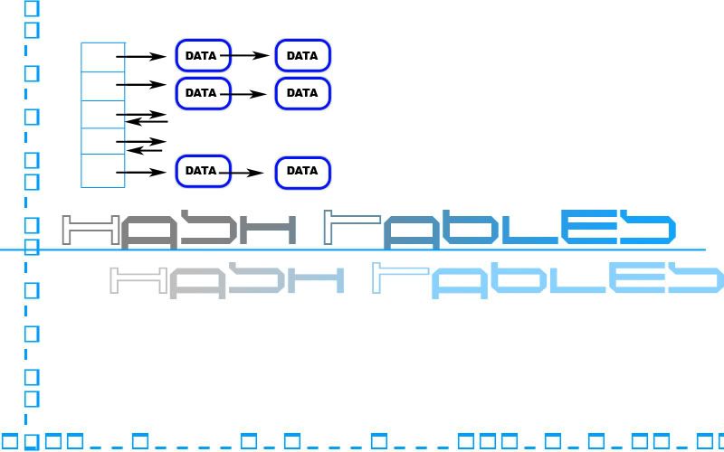
A hash table is a common data structure used for storing data which has a key/value relationship - we store data values in the hash table and access them through their keys. In its simplest form, a hash table consists of an array-based list and a hash function. A hash function is esentially an address calculator - it accepts a key as input and returns a hash value for that key. This hash value determines where the key's value should be stored. The hash value is an index which is compatible with the array-based list. We stored the value in the hash table at the address specified by the key's hash. This is an example of a rudimentary hash table; there are actually many types. A very common form of hash table involves storing linked lists of data at each position of an array-based list.
Example 1:
Given that student ID numbers are 7 digits in length, we could store student names in an array indexed by student ID numbers. Not only would this require a gargantuan amount of memory, but some student ID numbers could be obsolete, and thus, in declaring a huge array for every possible student ID number, we are setting aside space which we might never use. A better solution is to use a hash function, which can store data in a hash table of any size. In this case, a key is a student ID and its corresponding value is the name of that student. If we hash the key value, the hash function returns hash which tells us we should store the value in the hash table using the hash as an index. Each key has a unique value.
Example 2:
If we examine a hypothetical scenario where we are store data values in an array using keys as array indexes, we might have 10 key/value combinations and the largest key might be 99999. Using this approach, we would be forced to declare an enormous array of 99999 elements when we only want to actually store 10 elements in it. A hash function can take a large key and map it onto a hash table of any size - what this means is that a key of 99999 could be mapped onto a hash table with a storage range of 0-50 elements.
Hash tables have their downsides too. While they tend to be efficient data structures, in a worst case scenario, they can be incredibly slow and cripple a system.
This is an overview of the general hashing process:
1.) Convert our key into numeric form if it isn't already a number.
2.) Input our numeric key into the hash function which will output a hash value, dictating a desired destination of storage for our data value.
3.) Attempt to store our data value at the position indicated by the hash value. If there is already data present at that location, use a method of collision resolution to solve this problem.
In this section of the HTTB, we will cover many aspects of hashing such as...
Hash Functions 101 - The Role and Ideal Characteristics of Hash Functions
The role of a hash function is to take a numeric key, process it and return a hash value which dictates where we should store the key's data value. As mentioned above, a hash function can map a key/value combination of any sort onto a hash table of any size. If we want to map data onto a hash table of 100 elements, this can be achieved by using a hash function such as this, which makes use of the modulo function; hash(x) = x mod table_size, where table_size in this case is 100. Of course, this is an example of a very primitive hash function which is capable of mapping any numeric key onto any hash table. Any hash function will ideally be able to rapidly return a hash value, given a key.
Clearly by using this approach (and indeed any hashing function), it is possible to hash multiple keys to the same address, and this is known as a collision. Collision resolution is an area which deals with managing these collisions and is explained in greater depth below. Collisions are the major downfall of hashing as a collision slows down not only the storage of data, but also the retrieval of it. A perfect hash function can map each key to a unique address (index) in the hash table; i.e. i = hash(x). However, in reality, a perfect hash function can only be constructed if we know what data it will be used to store beforehand. And since collisions are inevitable, collision resolution is necessary, and hash functions must attempt to avoid causing collisions. How can we achieve this?
A hash function is less likely to cause collisions if it hashes data evenly throughout the table, so that there is a uniform spread of data. If the data input is random (all possible search keys have equal probability of being stored), the hash function should be able to spread the data evenly within the hash table. An ideal hash function adds entropy to the data it is storing, so that if the input data isn't random, it will still be stored as evenly as possible in the hash table. It is possible for systems to be compromised by feeding non-random input to a hash function, as that data will mostly hash to the same location and thus, collisions which require resolution will be rife (extra processing required to store/retrieve data). By spreading data evenly throughout the hash table and adding entropy to it, the frequency of collisions can be minimised. In the below examples, we will examine on a more intricate level, how rudimentary hash functions work.
Example 1: Using hash functions to store random data
Imagine we are storing the names of people in a hash table to be accessed by an 5 digit ID number as a key - and the ID numbers go from 0 to 40,999. One method of hashing these ID numbers might involve taking the first 2 digits of each number and hashing based on that. If we have a table size of 15 and use a hashing function of hash(x) = x mod table_size to hash all 40,999 ID numbers, we are effectively hashing random data which is evenly distributed. ID numbers starting with 00, 15 and 30 will be hashed to address 0 in the table while ID numbers starting with 14 and 29 will be hashed to address 14.
Effectively addresses 0-10 will hold 50% more data than addresses 11-14. This might not initially sound too dangerous, but the serious implication is that by the time we hash 40,999 numbers with that 50% imbalance, there will be 3000 data values stored at address 10 and 2000 data values stored at address 14. This kind of uneven data spread is what slows down hash tables during both storage and retrieval stages - this is an example of a poor hash function which fails to spread random data evenly.
Example 2: Using hash functions to store non-random data
Imagine we are creating a database of physics teachers around the world and storing their names as data values which are accessed by a 6 digit ID number as a key - and the ID numbers go from 0 to 150,000 where the first 3 digits of each number denotes the country in which the physicist currently lives. We might hash the data into a hash table with a size of 151 using hash(x) = (int) x / 1000, which effectively hashes each person to their country code. If we allocate 0 to 20,000 for Asian countries with 000 for China, 001 for India etc... and allocate 40,000 to 50,000 for Australasia, with 040 for Australia, 041 for NZ and 042 for Papua New Guinea, our input data will clearly be very skewed as there will be many data values stored at 000 and 001 due to the high populations of those countries, and barely any stored from 040 to 050.
Our hash function is storing data according to country code, and hence, isn't adding any entropy at all to the existing data. Since the input data is heavily skewed, the hash table distribution will also be very unevenly distributed, resulting in outrageous storage/retrieval times.
In summary, the ideal hash function spreads data evenly (both random and non-random (by adding entropy)) and executes efficiently itself.
Hash Tables Summary
- Hash Tables contain an Array-List of pointers that point to Linked Lists that contain data. Hash Tabls also include a Hash function.
- The Hash function takes in a key (input) and converts it into a number. It then performs a modulo operation with the size of the Array-based List backbone of the Hash table to return a unique index value.
- The modulo operation is used so that the potentially large and unusable number (by the Array-List backbone) is converted into a number that can be used as an index to the Array-List.
- Inevitably, the modulo operation may return the same number and thus values are mapped onto the Hash table at the same Array-List location.
- This is done by adding the new data node to the Linked List attached to the Array-List location in question.
- However, if a Linked List gets too long, the lookup time for the data nodes along this Linked List becomes very large.
- Hence it is ideal to have an even distribution of values produced by the Hash function.
- As more and more nodes are added, the number of Linked-Lists along any of the Array-List locations will grow regardless of a good or bad hash function.
- Thus the lookup time for data will increase inevitably.
- To battle this, a resizing operation of the Array-List takes place at a certain point. This is favourable as Array-Lists have constant lookup time unlike Linked Lists regardless of size.
- The point where the resizing operation is taken place is deemed by a certain "Load Factor".
- The Load Factor is the ratio between the number of Data Nodes and the Size of the Array-list. It is numerically represented as No. of Data Nodes/Size of Array-List.
- When the Load Factor gets too high, the array gets resized.
Common Hash Functions
Problems with Hashing
Occasionally, a collision occurs when two different keys hash into the same hash value and are assigned to the same array element. A common way to deal with a collision is to create a linked list of entries that have the same hash value. For example, say that the key of each entry hashes to the same hash value, and this results in both being assigned to the same array element of the hashtable. Because two entries cannot be assigned the same array element, a linked list is created. The first user-defined structure is assigned to the pointer in the array element. The second isn't assigned to any array element and is instead linked to the first user-defined structure, thereby forming a linked list.
Collision Resolution
Here is a screencast which is intended as a brief introduction to collision resolution methods such as linear probing, quadratic probing, double hashing and separate chaining. It is stored on the university intranet, and hence can only be accessed on campus.
Introduction to Collision Resolution
Collision Theory by hbar055
When two keys hash to the same position in a hash table, they collide. Chained hash tables have a simple solution for resolving collisions: elements are simply placed in the bucket where the collision occurs. One problem with this, however, is that if an excessive number of collisions occur at a specific position, a bucket becomes longer and longer. Thus, accessing its elements takes more and more time. Ideally, we would like all buckets to grow at the same rate so that they remain nearly the same size and as small as possible. In other words, the goal is to distribute elements about the table in as uniform and random a manner as possible. This theoretically perfect situation is known as uniform hashing; however, in practice it usually can only be approximated. Even assuming uniform hashing, performance degrades significantly if we make the number of buckets in the table small relative to the number of elements we plan to insert. In this situation, all of the buckets become longer and longer. Thus, it is important to pay close attention to a hash table’s load factor. The load factor of a hash table is defined as: n/m; where n is the number of elements in the table and m is the number of positions into which elements may be hashed. The load factor of a chained hash table indicates the maximum number of elements we can expect to encounter in a bucket, assuming uniform hashing. For example, in a chained hash table with m = 1699 buckets and a total of n = 3198 elements, the load factor of the table is a = 3198/1699 = 2. Therefore, in this case, we can expect to encounter no more than two elements while searching any one bucket. When the load factor of a table drops below 1, each position will probably contain no more than one element. Of course, since uniform hashing is only approximated, in actuality we end up encountering somewhat more or less than what the load factor suggests. How close we come to uniform hashing ultimately depends on how well we select our hash function.
Hash Functions Used in Lab 5
We used the following Hash Functions for our labs:
- BuzHash - a very good hash function, which I discovered was developed by one of our lecturers in uni, back in 1996.
- BuzHashn
- Hash_CRC
- Base256 - a bad hash function, does not introduce any sort of randomness into the keys, just converts the data into integers.
- Java_Integer - simply returns the integer value, works great for numbers.
- Java_Object
- Java_String
- Rand
- High_Rand
The Buzhash function is the best function as we saw it was observed in the labs. It gave very good results overall in the theoretical tests, and performed to expectations in the
practical tests.
Buzhash - algorithm that requires the use of a random table 256 words large, where a word is defined as the maximum data size that an XOR function
This function takes the input, xors each character with the value from the 256, while doing to the character's ascii value.
I tried to find some explanations for these hash functions via Google, and the top result I got was John Hamer's Notes from 2004.
Some Notes by El Pinto
Hashing Tables are data structures for storing elements for fast lookup.
A hash function is a function that generates a number from a string or other data value.
A hash table uses a hash function to allocate data space in the hash table and to minimize the number of collisions.
The problem is to find a good hash function which can avoid collisions as much as possible.
The statistics of a uniform random variable tells us what what a good hash function looks like.
A good hash function is one that gives us values that have been uniformly distributed, meaning there is no relationship between the elements.
The load factor is given by the number of elements divided by the number of bins in a hash table(the number of rows).
In practice, we have a whole family of hash tables for different types of data.
xor, has the ability to give us entirely random key for our input data, xor is what is used in buzhash function.
(Referenced from John Hamers notes, 2004)
Lab #5 - How Do Hash Functions Perform in Theory and in Practice?
Experiment 1 of Lab 5 involved feeding a sample size and data to a pseudo-hash function which performed various randomness tests using Poisson Theory. Here are details on some of the statistical tests used for measuring the randomness of hash functions.
Statistical Tests for Hash Functions
| Entropy | Entropy represents the information density of data and is measured in bits per byte. Presumably 'information' refers to
'unique information'. In other words, information density of data refers to the amount of unique non-redundant information per unit of data. A data source of low randomness has a low entropy because the information content is low as some of the information is repeated (the data has patterns) and thus, the information density is low. In a hashing context, an entropy value closer to 8 means that the hash function is theoretically more randomised. |
| Chi-square Test | The Chi-Square test is a commonly used tool for testing the randomness of data. It involves calculating the
chi-square distribution for the data and representing by an absolute number and a percentage which represents how frequently truly random data would exceed the absolute number calculated. Chi-square percentage values closer to 50% indicate data which is more random. Interpretations based on chi-square % (p) follow: Data is almost certainly non-random: p < 1% OR p > 99% |
| Arithmetic Mean | The arithmetic mean is calculated by adding all the byte values in the data and dividing by the length of the
data (in bytes). The expected mean is the halfway mark of the value range - since a byte can represent 0-255, the expected mean is 127.5. If the arithmetic mean is close to the expected mean, we can infer that the data is random. |
| Monte-Carlo Method for Pi | The Monte-Carlo Method for Pi evaluates each sequence of 24 bits, creates (x,y) coordinates for each one and plots it on a square
which has a circle inscribed inside it. Since the area of the circle is π*r^2 and the area of the square is 4r^2, then multiplying the circle area by 4 and dividing by the square area will give π. If we are plotting truly random points, then the proportion of points inside the circle to points outside the circle should be equal to the proportion of the respective areas and 4C/S (C = number of points inside circle, S = number of points inside square) should be close to π (also depends on number of points). So if we perform the Monte-Carlo test on random data, it will return the approximation of pi based on that data and a percentage error which shows the deviation of the approximation from the correct value. Obviously a smaller percentage error means that the data is more random. |
| Serial Correlation Coefficient | The serial correlation coefficient measures the degree of dependency between consecutive bytes in the data and can be positive or
negative. A value close to 0 indicates data which is more random. |
The Significance of Testing Hash Functions on both Low and Typical Entropy Sources is discussed in the screen cast provided.
Experiment 2 involved computationally estimating llps (length of longest probe sequence) values for each function and then measuring the actual llps values.
Hashing Efficiency
Screencast Directory for Hashing
Table with screencast descriptions shown below:
| User | Description |
|---|---|
| ssre005 | Significance of Testing Hash Functions on both Low and Typical Entropy Sources |
| jsmi233 | Motivation for Hash Tables |
| npit006 | A Brief Introduction to Collision Resolution |
| aomr001 | Introduction to Hash tables 1 |
| aomr001 | Introduction to hash tables 2 + chain length |
Resources / References
http://oopweb.com/Java/Documents/IntroToProgrammingUsingJava/Volume/c12/fig2.jpeg
Data Abstraction and Problem Solving With Java - Frank M. Carrano, Janet J. Prichard
http://www.fourmilab.ch/random/
Hash Tables Notes by John Hamer, 2004
http://www.partow.net/programming/hashfunctions/#HashAndPrimes
http://lists.trolltech.com/qt-interest/2002-01/thread00680-0.html
Exam Questions
2007 Exam Question 2 with Possible Solutions
a) Draw a Diagram of a hash table, clearly showing the relationship between all components of the structure and their arrangement in memory=====
http://oopweb.com/Java/Documents/IntroToProgrammingUsingJava/Volume/c12/fig2.jpeg
The array based list is a typical resizing array so the diagram implies that it is stored in a contiguous space in memory.
The linked lists are accessed by arrows which represent pointers to the next cell.
b) The "Load Factor" of a hash table is defined as the number of elements divided by the table size
i-Choosing a Load Factor involves a Tradeoff. What is this tradeoff?
The tradeoff is between the cost of using memory and the cost of time taken to resize an array.
ii-Traditionally, load factors of 0.5 or less were recommended for Hash Tables. More modern recommendations are up to 5 or more. What has led to this change??
If a hash table has a load factor of 0.5, this means that the number of data nodes/the size of the array = 0.5 which means the size of the array doubles the number of data nodes at this load factor. If a hash table has a load factor of 5 this means that the number of data nodes is 5 times bigger than the size of the array.
It seems that in the present, large load factors are used so that more favour is given to lessening the time consuming resizing operations and thus the reason for this change must be that these days, so much more memory is available such that the cost of memory is less of a concern.// My bad. I think the answer is just improved CPU speed lol! - Shrek
Improvements in processor speeds also makes lookup time along the linked lists of the Hash table less of a concern as well. Thus, linked lists in Hash tables getting too long also becomes less of a concern.
iii-How is a given load factor maintained when the number of elements in the table can vary??
When the array based list of the hash table is resized by a certain factor, the load factor reduces by that factor and thus, adding elements to the hash table allows for the load factor to return to that same value.
c) What are the requirements of a good hash function
A good hash function must create a unique index from a given input. The output indexes of the hash function must be uniformly distributed.
d) Why are hash chains typically implemented as singly linked lists, rather than array-based lists
So that memory for new data nodes is allocated in constant time and only the amount of memory that is needed is allocated.
e) What is the advantage in choosing a prime number of bins for a hash table when a good hash function (such as Buzhash) is used?
Bins = size of array-based list.
According to 'http://www.partow.net/programming/hashfunctions/#HashAndPrimes':
"There isn't much real mathematical work which can definitely prove the relationship between prime numbers and pseudo random number generators. Nevertheless, the best results have been found to include the use of prime numbers."
According to the results shown on 'http://lists.trolltech.com/qt-interest/2002-01/thread00680-0.html', using an array size that is a prime number increases the spread of index values produced by the modulo operation.